Often we run statistical code within one program. However, statistical programs may excel at some tasks but not others (e.g., like running complex models but not producing nice plots and tables). We may find situations where we want to take advantage of the best features of a set of programs. Alternatively, we may have staff with expertise in one program but need to use features in another. The following is a brief set of simple examples that illustrate ways to generate code, run code, and collect results in one program from another.
Executing Mplus via SAS
Suppose you want to run a Monte Carlo simulation using Mplus but want to do this across a set of conditions. You could do this by running Mplus several times across a small subset of conditions. Alternatively, you could automate this process using SAS (or R) to write Mplus code, run the code, gather the results, and generate tables and plots of the results.
For example the following code uses SAS IML to generate an Mplus .inp file iteratively across a set of macro variables. Then, X call is used to run the Mplus files. Afterwards, a data step (infile) is used to retrieve the results. Finally, the results are plotted using SAS proc sgplot.
Here is what it might look like:
First, define any macro variables by using a %LET statement.
%LET libpath = C:\Desktop\MonteCarlo_SIM_Simple_Mediation;
%LET rep = 1000;   *simulation reps;
%LET MIN_N = 100;  *sample size minimum;
%LET MAX_N = 120;  *sample size maximum;
%LET MIN_RSQ = 20; *effect size (R2) minimum (whole number only; e.g., 1 <-- .01);
%LET MAX_RSQ = 26; *effect size (R2) maximum (whole number only; e.g., 25 <-- .25);
%LET varX = .25;   *variance of X (.25 for binary variable with a 50/50 split);
%LET miss = .15;   *Percent MCAR missing data;
Next, a %macro statement is used to specify the name of the macro (“mplusSIM”). This macro takes arguments which are listed in parenthesis after the name of the macro (i.e., samplesize=, varX=, aR2=, bR2=, cR2=, and miss=) to pass macro variables into the code. Within mplusSIM macro variables are referenced with & (e.g., &samplesize). Here, varX is the variance of x, aR2 is the effect size for the regression of M on X, bR2 is the effect size for the regression of Y on M, and cR2 is the effect size for the regression of Y on X. miss is the percent of MCAR missingness (e.g., miss=.15 is 15% missing on M and Y).
%macro mplusSIM(samplesize=, varX=, aR2=, bR2=, cR2=, miss= );
Then, create any additional macro variables such as: beta for M regressed on X (MonX), beta for Y on M (YonM), and beta for Y on X (YonX) to achieve specificed effect size, implied correlation of X and M (rXM) based on MonX and the implied residual variance of M (Em), the residual variance of Y (Ey); or any summary statistics of interest such as the effect size (R2), percent of missing data, proportion of total effect mediated (Pm) and the ratio of indirect to the direct effect (Rid).
proc iml;
x mkdir "&&libpath";
Em = (1-(&aR2/100));
  call symput('Em',left(char(Em)));
MonX = sqrt(((1-Em)/&varX));
  call symput('MonX',left(char(MonX)));
YonM = sqrt((&bR2/100));
  call symput('YonM',left(char(YonM)));
YonX = sqrt((&cR2/100)/&varX);
  call symput('YonX',left(char(YonX)));
rXM = MonX*&varX;
  call symput('rXM',left(char(rXM)));
Ey = (1-(YonX**2*&varX)-(YonM**2)-(2*YonM*YonX*rXM));
  call symput('Ey',left(char(Ey)));
Pm = ((MonX*YonM)/(YonX+(MonX*YonM)));
  call symput('Pm',left(char(Pm)));
Rid = (Pm/(1-Pm));
  call symput('Rid',left(char(Rid)));
Now, create the Mplus .inp file using Proc IML referencing any macro variables.
file "&&libpath\med_&aR2._&bR2._&cR2._&samplesize._&miss._sim.inp";

put ("title: generate data");
put ("MONTECARLO:");
put ("names are x m y;        !Define variable names;");
put ("cutpoints = x (0);      !Define cutpoint to generate binary treatment;");
put ("NOBSERVATIONS = &samplesize ;");
put ("NREPS = &rep ;");
put ("SEED =  461981 ;");
put ("PATMISS = m(&miss) y(&miss) ;");
put ("PATPROBS = 1; ");
put;
put ("MODEL POPULATION:");
put ("[x@0];        !mean of x set to 0;");
put ("x*&varX;        !total variance of x;");
put ("[m-y@0];      !mean of m and y;");
put ("m*&Em; !residual variance of m;");
put ("y*&Ey; !residual variance of y;");
put ("m on x*&MonX; !a path;");
put ("y on m*&YonM; !b path;");
put ("y on x*&YonX; !c' path;");
put;
put ("MODEL:");
put ("[m-y@0];        !mean of m and y;");
put ("m*&Em; !residual variance of m;");
put ("y*&Ey; !residual variance of y;");
put ("m on x*&MonX; !a path;");
put ("y on m*&YonM; !b path;");
put ("y on x*&YonX; !c' path;");
put;
put ("MODEL INDIRECT: !MODEL INDIRECT statement to obtain mediated effect;");
put ("y IND x;        !Start and endpoint of mediation model defined here;");
put;
put(" output:");
closefile  "&&libpath\med_&aR2._&bR2._&cR2._&samplesize._&miss._sim.inp";
Then, run the Mplus .inp files
X call "C:\Program Files\Mplus\mplus.exe"
           "&&libpath\med_&aR2._&bR2._&cR2._&samplesize._&miss._sim.inp"
	          "&&libpath\med_&aR2._&bR2._&cR2._&samplesize._&miss._sim.out";
Next, read results from the MPLUS .out files into SAS
data PARAMS.TOTind;
infile "&&libpath\med_&aR2._&bR2._&cR2._&samplesize._&miss._sim.out";
input @'Tot indirect' Population Average StdDev SEavg MSE COVER POWER;
Run;
End Macro
%mend mplusSIM;
SAS MACRO to iterate through various sample sizes and effect sizes
%macro samplesize;
%do h=&MIN_N %to &MAX_N %by 10;
  %do j=&MIN_RSQ %to &MAX_RSQ %by 1;
%mplussyntaxpop(varX=.25, aR2=&j., bR2=&j., cR2=&j., samplesize=&h., miss=&miss.);
   %end;
 %end;
End macro
%mend samplesize;
Run simulation
%samplesize;
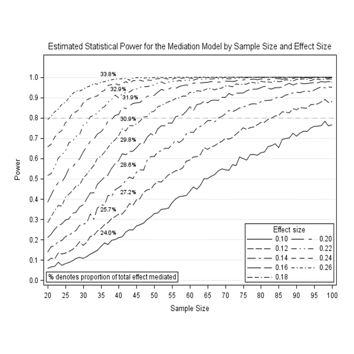
Plot the power curves (e.g., sgplot)
proc sgplot data=test;
where R2 in (.20,.22,.24,.26) ;
series y=power x=samplesize / group=R2 datalabel=pm1;
xaxis label='Sample Size' values=(20 to 100 by 5);
yaxis label='Power' grid offsetmax=.1 values=(0 to 1 by .10);
refline .80 / axis=y lineattrs=(pattern=dash) TRANSPARENCY = 0.5;
keylegend/ title='Effect size' location=inside position=bottomright down=5;
title 'Estimated Statistical Power for the Mediation Model by Sample Size and Effect Size';
INSET '% denotes proportion of total effect mediated'/ POSITION = BOTTOMleft BORDER;
run;
Here is the example plot:
Executing SAS via RMarkdown (export to Word)
Suppose you want to run a data analyses while also documenting the data and software code used so that others may verify the work. You could do this by running SAS code (including calling SAS macros) from R. For exmaple, first create an Rmarkdown document in RStudio. THe header might look like this:
---
title: "My data analysis"
author: "my name here"
date: "`r format(Sys.Date(), '%B %Y')`"
output:
  word_document: default
  html_document:
    df_print: paged
  pdf_document: default
---
Next, use the SASmarkdown package to point R to the sas.exe file inorder to run SAS code within R.
```{r setup, include=FALSE}

knitr::opts_chunk$set(echo = TRUE)
library(SASmarkdown)

saspath <- "C:/Program Files/SASHome/SASFoundation/9.4/sas.exe"
sasopts <- "-nosplash -ls 75"

knitr::opts_chunk$set(engine='sas', engine.path=saspath,
                      engine.opts=sasopts, comment="")
```
You can then specify code just like you would do for R - only be sure to use {sas name} rather than {r name} like this:
```{sas myregression}
proc glm data=mydata;
model myDV = myiv1 myiv2 myiv3 myiv4;
run; quit;
```
We could even export the results and pipe them into a text results writeup something like this:
```{sas myregression, collectcode=TRUE, include = FALSE}
proc glm data=mydata;
model myDV = myiv1 myiv2 myiv3 myiv4 /solution;
ods output ParameterEstimates=dPara;
ods output NObs=dNum;
ods output FitStatistics=dRsq;
ods output OverallANOVA=anova;
ods output ModelANOVA=myresults;
run; quit;

data _null_ ;
  set dNum;
    call symput("N",N);
run;

data _null_ ;
  set Drsq;
    call symput("RSquare",round(RSquare, .01));
    call symput("RSquarePCT", put(round(RSquare, .01), percent8.1));
run;

data _null_ ;
  set anova;
    if Source NE "Model" then delete;
    call symput("FValue", round(FValue, .01));
    call symput("DFnum", DF);
    call symput("ProbF", ProbF);
    call symput("ProbF", Put( ProbF, pvalue6.3));
    call symput("DV", Dependent);
run;

data anova; set anova;
beta = byte(223); *222;
*beta = {unicode beta};
rsq=byte(178);
run;

data _null_ ;
  set anova;
    if Source NE "Error" then delete;
    call symput("DFden", DF);
    call symput("r2", rsq);
    call symput("beta", beta);
run;

data mycounts ;
  set dpara;
  array a Probt:;
  array values{1} Probt;
  do i=1 to dim(a);
    if values{i} < 0.05 then sig_count=sum(sig_count, 1);
  end;
    where NOT(Parameter EQ "Intercept");
run;

proc sql noprint;
 select sum(sig_count)
 into :SumList separated by ' '
 from mycounts
 where Probt < .05;
quit;

proc sql noprint;
 select Parameter into :ParamList separated by ' '
 from mycounts
 where Probt < .05;
quit;

 proc sql noprint;
 select Parameter, round(Estimate, .01), put(Probt, pvalue6.3)
 into :ParamList separated by ', '
      ,:EstList separated by ', '
      ,:PVList separated by ', '
 from mycounts
 where Probt < .05;
quit;
```
And now calling the collectcode from above and using proc odstext to print results:
```{sashtml mywriteup, echo=FALSE}
proc odstext;
p "Results" /style=[fontsize=14pt fontfamily=Arial ];
p "The multiple regression model with all predictors explained, &RSquarePCT of the
variance in &DV (R&r2 = &RSquare, F(&DFnum, &DFden) = &FValue, &ProbF). Results indicate
that &SumList of the predictors are significant with a sample size of N = &N.. Specifically,
we found that &ParamList significantly predicted &DV (b = &EstList, p = &PVList; respectively)."
/style=[fontsize=12pt fontfamily=Arial ];
run;
```
Example result in Rmarkdown:
/* Analysis code */
proc glm data=myBIDD;
model bisciscor = ASDgrp Cgender income Cage /ss3 ;
run; quit;

/* Results */
                             The GLM Procedure

                  Number of Observations Read         258
                  Number of Observations Used         228

 Error                    223    5479.08525      24.56989

 Corrected Total          227   14561.36842

          R-Square     Coeff Var      Root MSE    bisciscor Mean

          0.623725      41.12631      4.956802          12.05263


 Source                    DF   Type III SS   Mean Square  F Value  Pr > F

 myiv1                      1   7916.176924   7916.176924   322.19  <.0001
 myiv2                      1     12.583286     12.583286     0.51  0.4750
 myiv3                      1     63.566923     63.566923     2.59  0.1091
 myiv4                      1     85.923447     85.923447     3.50  0.0628

                                       Standard
     Parameter         Estimate           Error    t Value    Pr > |t|

     Intercept       8.38611270      1.75118904       4.79      <.0001
     myiv1          12.49003158      0.69583679      17.95      <.0001
     myiv2          -0.55446027      0.77477394      -0.72      0.4750
     myiv3          -0.41721340      0.25938464      -1.61      0.1091
     myiv4          -0.16774353      0.08969981      -1.87      0.0628
The multiple regression model with all predictors explained, 62.0% of the variance in
myDV (R² = 0.62, F( 4, 223) = 92.41, <.001). Results indicate that 1 of the predictors
was significant with a sample size of N = 228. Specifically, we found that myiv3
significantly predicted myDV (b = 12.49, p = <.001).
Executing SAS and/or Mplus via R (without a dedicated package)
We could also write and run SAS or Mplus code using R without using an R package. Consider…