Missing data is really an incredible area of research. It occurs in most areas of the applied sciences and knowledge of missing data can function sort of as a repair kit - so that you can avoid losing additional information when handling missingness. We can actually use missing data theory when designing studies to decrease participant burden and research costs.

But that’s not what I want to mention here, because right now most statistical software programs have defaults that do not properly deal with missing data. So let’s review one of these often neglected missing data handling concepts and look at some examples - all of which are available for download so that you can test out these ideas for yourself.

For those of you interested in further reading on the topics discussed today, I recommend John Graham’s article “missing data analysis: making it work in the real world” – as the title suggests this is written with applied researchers in mind and I love that it covers a wide range of important issues.

Missing Data Mechanisms

While patterns describe where data are missing, causes describe why data are missing. Discussion now turns to what causes missing data because it is helpful to know what kind of missing data introduces error into your analyses.

The literature describes 3 basic types of missing data mechanisms and they are MCAR, MAR and MNAR. This is a diagram of the missing data mechanisms that illustrates each can contribute to the missing data you have on your dataset.

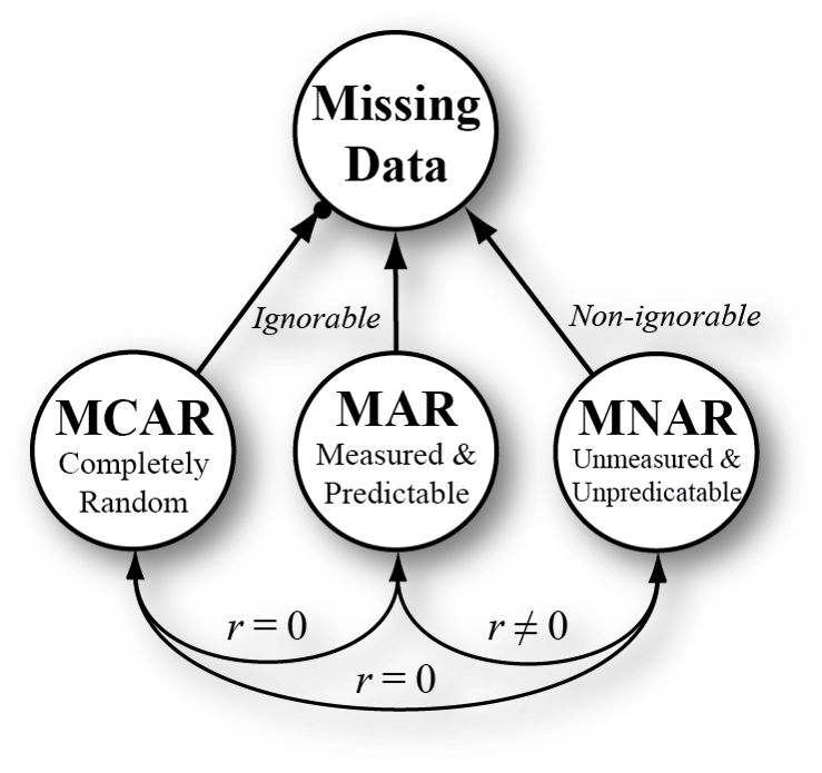The first mechanism is called Missing Completely at Random (MCAR). This means that the data are missing due to a random process. All missing data procedures assume at least this level of missing data. So, if you do traditional techniques like: pairwise deletion, listwise deletion, and so on – which are often the software defaults - you assume that the data were MCAR. This is not a great assumption.

Now where modern missing data handling tools come in handy is when the data are missing at random (MAR). This means the data are missing for a reason and we have a variable that is assoicated with the missing data.

Suppose that data are missing because of low socioeconomic status (SES) and I happened to measure SES in my dataset. If so I can do a good job of recovering the missing information. The reason this works is because I know what a low SES person would look like on the missing scores because I had some that stayed in and I also know what the relationships are among all the other variables.

The third mechanism is the Missing Not At Random (MNAR). What this one means is that there is a reason for the missing data and unfortunately we don’t have a measure of it. This is the drawback of any missing data. If there is a reason and we don’t have a measure of it – then our ability to recover that information is severely limited. That’s why this is referred to as non-ignorable missing data.


Consider example data to illustrate basic missing data handling techniques.

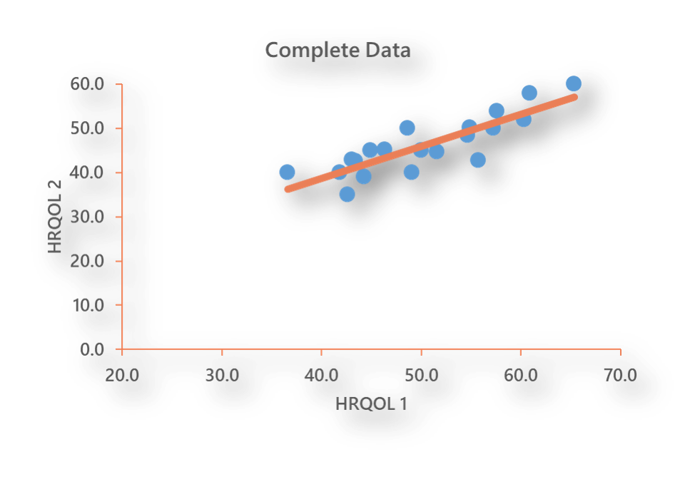
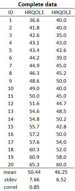
This is the scatter plot of the correlation between the HRQOL1 and HRQOL2 variables without any missing values.

Now lets impose the missing data and estimate the correlation using listwise deletion.

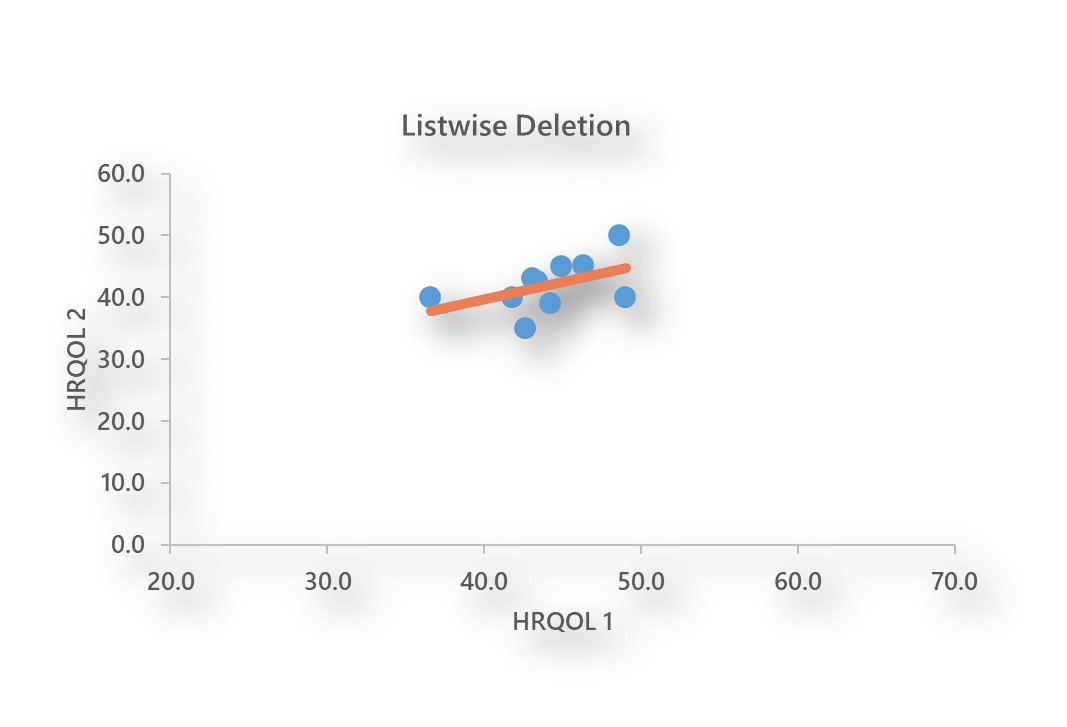
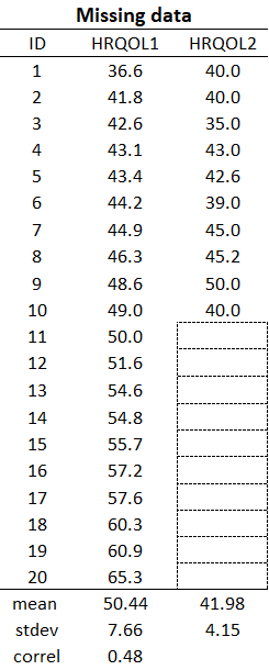
To demonstrate the bias that results from complete cases analysis I deleted scores on HRQOL2 if HRQOL1 was > = 50. Using listwise deletion the last 9 participants would be deleted.

As you can see, this scatter plot looks very different than the original. Here, half the data were deleted and the estimation is incorrect. As we will see shortly, it is actually possible to get back the lost information when the correct approach is used to properly account for the missing data. Remember that the HRQOL1 variable was responsible for creating the missing data.