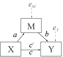
In statistical analysis, mediation refers to the process through
which one variable mediates or explains the relationship between two
other variables. This concept is crucial in various fields, including
psychology, social sciences, and epidemiology, where researchers often
need to understand the mechanisms underlying observed relationships.
In this blog post, we’ll explore a piece of R code that performs a
simple mediation analysis and generates power curves to assess the
statistical power of the mediation model under different conditions.
Main Analysis Loop
for (N in n_list){
  for (a in a_list){
    for (cprime in c_list){
      b <- a

      # ... (rest of the loop)

      # Store results in the 'w' variable
      w = rbind(w, c(N, a, b, cprime, R2_a, R2_b, Pm, Mrat, power))

      # ... (rest of the loop)
    }
  }
}
This loop iterates through various combinations of sample sizes (N),
values of ‘a’, and ‘cprime.’ It calculates statistical power for a
simple mediation model, stores the results in the ‘w’ variable, and
extracts other relevant statistics like R-squared (R2_a, R2_b),
proportion mediated (Pm), and more.
Full code
library(MASS) # for the sampling
library(tidyverse) # for the plot
library(lavaan) # for the R2
library(plyr)
myfiles <- dirname(rstudioapi::getSourceEditorContext()$path)
#windowsFonts(`Segoe UI` = windowsFont('Segoe UI'))
# Simple mediation --------------------------------------
w = NULL # We want to store results in here
mcmcReps <- 10000
seed <- 461981
powReps <- 2000
conf <- 95 #----Confidence Level (%)
n_list = c(seq(50, 300, by = 10)) #sample size
#a_list = c(.17, .22, .26, .30, .33, .45, .50) #seq(.10, .50, by = .02))
a_list = c(0.14, 0.20, 0.26, 0.30, 0.39) #0.14, 0.26, 0.39, 0.59
#b_list = c(.39)
c_list = c(.39)
SDX <- 1
SDM <- 1
SDY <- 1
for (N in n_list){
for (a in a_list){
# for (b in b_list){ #change to b_list
for (cprime in c_list){
b <- a
print(paste0("N=", N, " b=", b, " Time=", Sys.time())) # track progress - this takes some time to run.
# Create correlation matrix
corMat <- diag(3)
corMat[2,1] <- a
corMat[1,2] <- a
corMat[3,1] <- a*b + cprime
corMat[1,3] <- a*b + cprime
corMat[2,3] <- b + a*cprime
corMat[3,2] <- b + a*cprime
# Get diagonal matrix of SDs
SDs <- diag(c(SDX, SDM, SDY))
# Convert to covariance matrix
covMat <- SDs %*% corMat %*% SDs
#--- OBJECTIVE == CHOOSE N, CALCULATE POWER -----------------------------------#
# Create function for 1 rep
powRep <- function(seed = 1234, Ns = N, covMatp = covMat){
#set.seed(seed)
dat <- mvrnorm(Ns, mu = c(0,0,0), Sigma = covMatp)
# Run regressions
m1 <- lm(dat[,2] ~ dat[,1])
m2 <- lm(dat[,3] ~ dat[,2] + dat[,1])
# Output parameter estimates and standard errors
pest <- c(coef(m1)[2], coef(m2)[2])
covmat <- diag(c((diag(vcov(m1)))[2],
(diag(vcov(m2)))[2]))
# Simulate draws of a, b from multivariate normal distribution
mcmc <- mvrnorm(1000, pest, covmat, empirical = FALSE)
ab <- mcmc[, 1] * mcmc[, 2]
# Calculate confidence intervals
low <- (1 - (conf / 100)) / 2
upp <- ((1 - conf / 100) / 2) + (conf / 100)
LL <- quantile(ab, low)
UL <- quantile(ab, upp)
# Is rep significant?
LL*UL > 0
}
set.seed(seed)
# Calculate Power
pow <- lapply(sample(1:2000, powReps), powRep)
# Output results data frame
df <- data.frame("Parameter" = "ab",
"N" = N,
"Power" = sum(unlist(pow)) / powReps)
power<-df$Power
###--------------- get R2 -------------------------###
n_cov <- nrow(covMat)
colnames(covMat) <- c("C1","C2","C3")
rownames(covMat) <- c("C1","C2","C3")
fitb <- lavaan::sem("C3 ~ C1 + C2", sample.cov = covMat,
sample.nobs = n_cov)
R2_b <- inspect(fitb, 'r2') # r-squared
fita <- lavaan::sem("C2 ~ C1", sample.cov = covMat,
sample.nobs = n_cov)
R2_a <- inspect(fita, 'r2') # r-squared
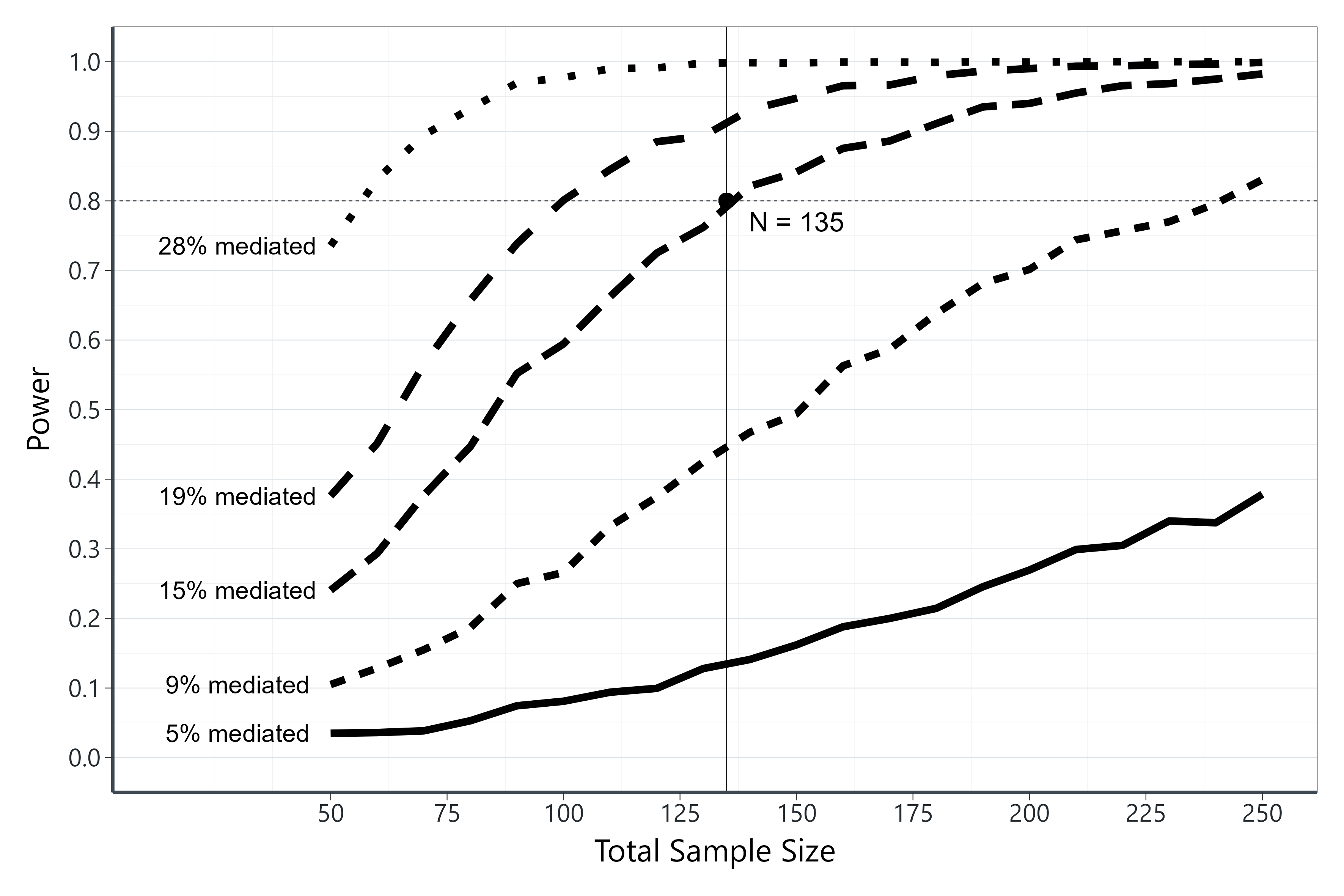
Pm <- (((a*b)/(cprime+(a*b)))*100) # as a %
Mrat <- Pm/(1-Pm)
w = rbind(w, c(N, a, b, cprime, R2_a, R2_b, Pm, Mrat, power))
colnames(w) = c('n', 'a', 'b', 'cprime', 'r2a', 'r2b', 'Pm', 'Mrat', 'Power')
simdf <- as.data.frame(w)
simdf$grpa <- as.factor(round(simdf$r2a, 2))
simdf$grpb <- as.factor(round(simdf$r2b, 2))
simdf$grpc <- as.factor(round(simdf$Pm, 0)) # Proportion of total effect mediated (Pm)
simdf$grpd <- as.factor(round(simdf$Mrat, 2)) # Ratio of indirect to the direct effect
# }
}
}
}
newdata <- simdf
p <- ggplot(newdata, aes(x = n, y = Power, group = grpa, linetype = grpa)) + #or color = grp
geom_line(size = 4) + #geom_line(aes(linetype=grp))+
geom_hline(yintercept = .8, linetype = 2) +
# Add labels at the end of the line
#geom_text(data = filter(newdata, n == min(n)),
# aes(label = paste0(grp)),
# hjust = .5, nudge_x = -7, size=6) +
geom_text(data = filter(newdata, n == min(n)),
aes(label = paste0(grpc, "% mediated")),
hjust = .5, nudge_x = -25, size=11) +
# Allow labels to bleed past the canvas boundaries
coord_cartesian(clip = 'off') +
scale_x_continuous(breaks=(seq(min(n_list), max(n_list), by = 50)), limits = c(min(n_list)-40, max(n_list))) +
scale_y_continuous(breaks=(seq(0, 1, .10)), limits = c(0, 1)) +
geom_vline(xintercept = as.numeric(round(simdf$n[which(diff(simdf$Power > .7999)!=0 & simdf$Pm == min(simdf$Pm) )],0)[1]) ) + #Target sample size
geom_point(aes(x=as.numeric(round(simdf$n[which(diff(simdf$Power > .7999)!=0 & simdf$Pm == min(simdf$Pm) )],0)[1]), y=.80), colour="black", size=6)+
annotate("text", x = as.numeric(round(simdf$n[which(diff(simdf$Power > .7999)!=0 & simdf$Pm == min(simdf$Pm) )],0)[1])+12, y = .77, label = paste0("N = ", as.numeric(round(simdf$n[which(diff(simdf$Power > .7999)!=0 & simdf$Pm == min(simdf$Pm) )],0)[1])), size=10)+
labs(x = "Total Sample Size", y = "Power")+
theme_bw()
p + theme(legend.position='none',
text = element_text(family = "Segoe UI"),
plot.margin = unit(rep(1.2, 4), "cm"),
plot.title = element_text(size = 20,
color = "#22292F",
face = c("plain"),
margin = margin(b = 5)),
plot.subtitle = element_text(size = 15,
margin = margin(b = 35)),
plot.caption = element_text(size = 10,
margin = margin(t = 25),
color = "#606F7B"),
panel.background = element_blank(),
axis.text = element_text(size = 24, color = "#22292F"),
axis.text.x = element_text(margin = margin(t = 5), size= c(32)),
axis.text.y = element_text(margin = margin(r = 5), size= c(32)),
axis.line = element_line(color = "#3D4852", size = 2),
axis.title = element_text(size = 40),
axis.title.y = element_text(margin = margin(r = 15),
hjust = 0.5),
axis.title.x = element_text(margin = margin(t = 15),
hjust = 0.5),
axis.ticks.length=unit(.35, "cm"),
panel.grid.major = element_line(color = "#DAE1E7"),
panel.grid.major.x = element_blank()
)
ggsave(paste0("/", format(Sys.time(), '%Y %B %d'), "mediation power curves.tiff"), path = myfiles, width = 60, height = 40, units = "cm", dpi=300)
urlplot <- paste0(myfiles, "/", format(Sys.time(), '%Y %B %d'), " mediation power curves.tiff")